|
Definition If there exists a neighbourhood of z0 throughout which f is analytic except at z0 itself, then z0 is an isolated singularity of f. Example Contrast Log z which has a continuous ray of singularities. Now from the Cauchy integral formula and the Derivative formulae,
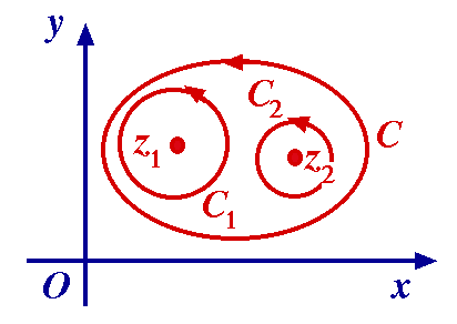
where the integrals are in an anti-clockwise direction about a simple closed contour containing z0. We observe that the values of these integrals are of the form 2 We now change our notation, replacing f(z) / (z – z0) by f(z). Then Definition Theorem 7.1 (Residue Theorem) Let C be a closed contour within and on which function f is analytic except for a finite number of singular points z1, z2, ... , zn interior to C. If Ki denotes the residue of f at zi, then
where the integral is around C in positive sense. Proof Let each zi be enclosed as shown in a circle Ci with radius small enough so that C and Ci are all separated. Now f is analytic in the remaining region within and including C, so by Cauchy's Theorem:
so using the definition of Ki. It follows that evaluation of such integrals depends on our ability to evaluate residues. Evaluate The singularities inside C are z = 0, 1. So I = 2 Find K0. Set g(z) = (5z – 2)/(z – 1) – analytic in a small circle C0 centred at 0. By the Cauchy integral formula, Find K1. Set h(z) = (5z – 2)/z – analytic in a small circle C1 centred at 1. Again by the Cauchy integral formula, Hence I = 2 (1) Use partial fractions:
(2) Use the Laurent expansion with | z | > 1, and find the coefficient of 1/z. So
and noting that the coefficient of 1/z is 5, we obtain the result as before. Singularities are obviously important in the theory. The nature of a singularity can be determined from the Laurent expansion
and in particular from the portion involving negative powers, known as the principal part of f at z0. Suppose f(z) = Then f has a pole of order m at z0 (or z0 is a pole). (1) Consider f(z) = (z2 – 2z + 3) / (z – 2). Now (2) Consider f(z) = (z + 1)/(z2 + 1)2 and z = –i. Set
(3) Consider f(z) = sin z / z . Here
We say z = 0 is a removable singularity. We could define f(0) = 1. (This would give a new function, coinciding with f for z (4) Consider f(z) = e1/z. There is a problem here at z = 0. Assuming
it is not possible to put this in the form (5) Essential singularities often exhibit strange behaviour. When f has a pole at z0, we expect f(z)
(1) We can give general formulae for the residues for poles of order m – essentially using Theorems 6.3, 6.4. (2) Work on series is useful here. (3) Most examples treat poles of low order. It is suggested that you learn the Cauchy integral formula and the Rules on Differentiation with respect to z0. Thus: (1) Consider This function has a pole of order 3 at z = 0. (2) Consider This function has a simple pole at z = 3i.
In the case of real improper integrals, we make the definition:
where both integrals on the right exist. Notice that the variables R, R' tend to infinity independently in the two integrals. It is useful to define the Cauchy Principal Value (Cauchy P.V.) in the following way:
So with the Cauchy P.V., we are insisting that the upper and lower infinite limits are approached at the same rate. If the improper integral defined by (1) converges, then the value obtained is the Cauchy P.V. On the other hand, the Cauchy P.V. may exist and integral (1) not converge. Example Let f(x) = x. Here the Cauchy P.V. is 0, but the integral is not convergent. Special case If f is even and the Cauchy P.V. exists, then For in this case
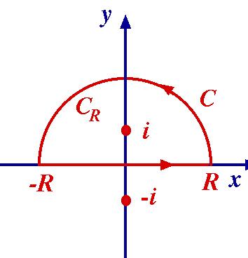
and the existence of the last Cauchy P.V. guarantees the existence of the first two integrals. Example If f(x) = p(x) / q(x) where p, q are real polynomials with no common factors, q(x) has no real zeros, and the degree of q(x) is greater than or equal to the degree of p(x) + 2, then Evaluate This has simple poles z =
For z = 2i: Hence
Now on CR,
and the length of CR is
So Question Is this easier than factorizing and using partial fractions in the real case?! Probably yes, especially as the integral around CR will fairly clearly always vanish when the difference in degree is 2 or more. Residue theory is also useful for evaluating integrals of the form
where p, q are real polynomials and q(x) has no real zeros. Note that the previous method cannot be used here. For we have | sin z |2 = sin2 x + sinh2 y and | cos z |2 = cos2 x + sinh2 y, so | cos z | and | sin z | increase like sinh y as y However, the integrals (*) can be combined to give
and | e iz | = e – y, which is bounded in the upper half plane. Show that This integral is the real part of
Now We show that the second integral tends to 0 as R | z2 + 1 |2 so Hence
So, taking real parts,
Since the integrand is even here, this Cauchy P.V. is the required integral. We can use residues to evaluate certain definite integrals of the type The variation of
and the integral becomes
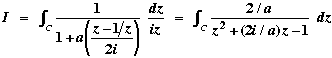
That is, a contour integral of a function of z around the circle C in the positive sense. Show that The formula is valid for a = 0. Suppose that a
where C is the circle | z | = 1 traversed in the positive direction. The denominator has zeros:
Hence the integrand is Also, noting that | a | > 1, we have | z2 | = (1 + that is, z2 lies outside C. Further, | z1z2 | = 1, so | z1 | < 1, – a simple pole inside C. The corresponding residue K1 is:
Hence I = 2
Because of time constraints, the course finished here. With a little more time, we would have showed that analytic mappings are conformal (preserve angle measure), and worked through a few boundary value problems. These would have demonstrated again the practical nature of complex analysis, and given us practice in the use of complex mappings.
|
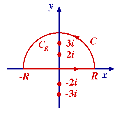 For z = 3i:
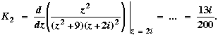
 So
So 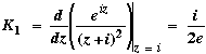 (calculating).
 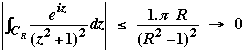 as R
as R