6. JULIA SETS
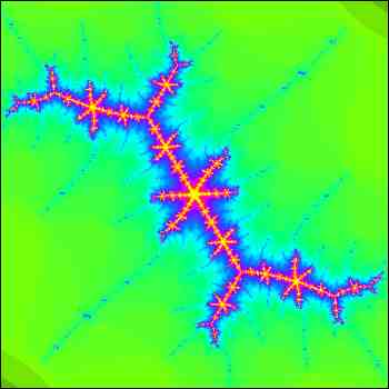
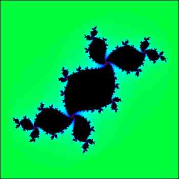
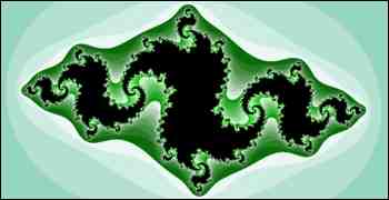
 Gaston Julia Gaston JuliaGaston Julia was a French mathematician who lived from 1893 to 1978. He is remembered today for the fractal sets which bear his name, the Julia sets. It is interesting how he came to study these sets. He had been looking at some work of Sir Arthur Cayley called ‘The Newton-Fourier Imaginary Problem’ about finding the roots of the equation f(z) = z3 + c = 0 using a method of iteration. He wondered if one could predict which of the three roots a given starting value of z would reach as a limit. The details are not important to us here, and we know that Julia found the solution to the problem difficult As with the Mandelbrot set, to understand the Julia sets, we need to understand complex numbers – the numbers of the form z = x + iy where x, y are real, and i2 = –1. Number z can be represented in the complex plane by the point (x, y). z It turns out that this sequence of points does one of two things. Either Now for any given value of c, we define the Julia set Jc to be the set of points z in the complex plane which never escape. Here are some examples (above right and below):
In each of these figures, the actual Julia set is designated in black, although this is obvious in only one of the figures. Normally when a Julia set is constructed, there is a system of colouring. Points which never escape are coloured black. Other points of the plane are coloured according to the speed with which they escape. This is done by choosing a large circle centred at the origin, and counting the number of iterations it takes for a point to get beyond this circle. The result of this process is particularly evident in the top diagram above, looking at the shades of green in the background. Where black points are not evident in a Julia set, they are revealed by zooming in on the set, looking at it with a greater magnification.
As mentioned above, the Mandelbrot set gives a wonderful way of classifying the Julia sets. We can explore this using the very neat applet devised by Rowan Seymour and used here with his permission. This applet appears on the web site and the author can be contacted at rowanseymour@gmail.com . Rowan recently obtained his PhD in Audio-visual Speech and Speaker Recognition from Queen's University Belfast, and is shortly going out to Rwanda to train computer programmers there. Place the applet window in the upper right corner of your screen so that it is visible while you work through the text. We notice that a Mandelbrot set appears in the left frame and a Julia set in the right frame. In each window the centre point is marked with a cross. The Mandelbrot or Julia set can be moved relative to this cross by dragging with the mouse, or using the arrow keys. Clicking on a frame activates it. There are various other controls. This applet gives us an excellent way of determining the relationship between the Mandelbrot set and the various Julia sets.
• In the applet, place the cross, c, within the Mandelbrot set, M. Describe the corresponding Julia set, Jc. What property of Jc appears to remain constant while c is in M? What happens when point c lies outside M? What happens if c lies near the border of M? (You might like to try zooming in on M while looking at this.)
But there is much more detail than this! • Compare the Julia sets Jc for points c in the main cardioid body of M and points c in the large circular disk to the left of the cardioid. In the latter case, notice how many solid regions meet at a common vertex. Now look at the Julia sets Jc for points c in the circular disk atop the cardioid. For these Julia sets, how many regions meet at a vertex? Now do some exploring on your own.
This is just a small sample of the relationships between the sets M and Jc . And while the mathematics is very interesting, don't lose sight of just how beautiful these sets are!
Fractals for the Classroom, Peitgen, H-O., Jürgens, H., Saupe, D. (Springer-Verlag 1992) |
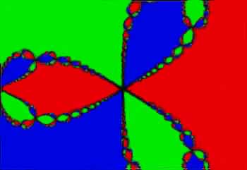 – not surprising in an age before computers! Today we know that there are ‘basins of attraction’, and these basins are infinitely complex. These basins for f(z) = z3 – 1 = 0, coloured red, blue and green, are pictured at left. This figure is a fractal, and is also an example of a Julia set.
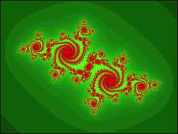 Now if c is a fixed complex number in the z-plane, let us consider the transformation of the plane under the mapping z