|

|
|
|
|
Coordinate systems In the last section, we considered complex numbers of the form x+iy, and we saw how such numbers could be interpreted as points in the complex plane. The real and imaginary components of the number correspond to the x– and y–coordinates of the associated point. Such x– and y–coordinates are called Cartesian coordinates. Each point in the plane is uniquely identified by its Cartesian coordinates. Cartesian coordinates are not the only possibility. We can also use polar coordinates, (r, |
It is possible to calculate each type of coordinates from the other, using the relationships:
x = r.cos 1. Work out formulae for calculating r and
|
 If the point P represents a complex number z = x + iy, then the polar coordinates of P are called the modulus and the argument of z. We met the modulus in the last chapter in its usual notation of |z|. The argument is usually written arg(z).
|
|
|||||||||||||
|
|
||||||||||||
|
|
|||||
|
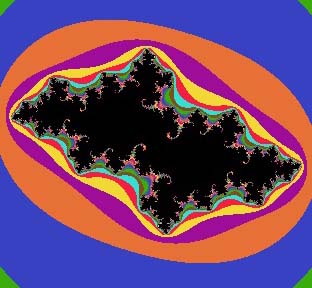
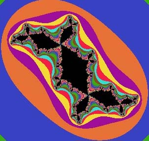
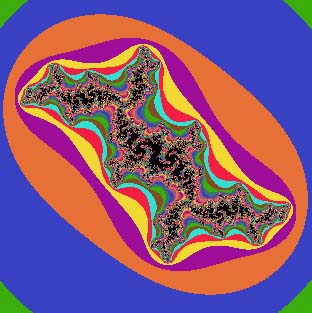
Some Julia sets are connected (all black areas are connected in one piece, as below; some are disconnected (with separate ‘islands’ of black). Can we tell from given complex number c, if J(c) is connected or not? The Mandelbrot set helps answer this question.
|
||||
|
|
|
|
Julia sets(II)
View the Julia sets: 4. Check the values of c associated with these Julia sets in an image of the Mandelbrot set. Are they in the Mandelbrot set or not? You may need to use a calculator to check. Do you think there might be a relationship between c being in the Mandelbrot set and J(c) being connected? 5. A small change in c can produce a big change in the appearance of J(c). In the group of images given above, for example, compare the sets J(0.25) and J(0.26). Use your program to explore the region between these values of c, to discover where and how this change occurs. |
The following program is very similar to the previous one for the Mandelbrot set. Procedures while and dot, again used in this program, are not given here, but need to be included.
|
|
|
|||
The program
|
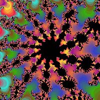
The program generates the illustrated Julia set, J(-0.27+1.04i). To obtain other Julia sets, allot different parameters in the last line.
|
||
|
|
|||
|
Julia sets and the Mandelbrot set Since they have the same generating formula, it should not be surprising that there are many interesting relationships between Julia sets and the Mandelbrot set. The Mandelbrot set can be defined as the set of points in the complex plane for which the associated Julia set is connected. A further connection is more profound. The Mandelbrot set contains, in a sense, a copy of every Julia set. Given a particular complex value c, the Julia set J(c) around the point z = c, on magnification, yields essentially the same image as the Mandelbrot set magnified around point c. 6. Choose a magnified image of the Mandelbrot set, for which you know the coordinates of the centre, c. Generate the Julia set for this value of c. What characteristics do the two pictures have in common? |
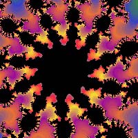
For example, the left picture shows a magnification of the Mandelbrot set around the point c = –0.724102 + 0.286462i. Note the 11-bladed ‘fan’ structure. The right picture is a magnification of the Julia set J(c) around the point z = c. Except for scaling and rotation, it looks the same as the first picture. This happens for every point on the boundary of the Mandelbrot set. The Mandelbrot set can be regarded as a catalogue of the Julia sets.
|
||
|
|
|
|
Further investigations 7. The last two chapters have discussed complex multiplication, but not division. Let us work out a formula for the result of dividing one complex number by another, in terms of the components of the two original numbers. Let the two numbers be z = x + iy and w = u + iv. The expression for z/w is easily obtained: The problem is to separate the real and imaginary components of the expression. Start the process by multiplying both the numerator and denominator by u – iv. This number is called the complex conjugate of w. |
8. (Harder) There are Julia Sets based on other functions besides z2+c. One class of attractive symmetrical Julia Sets is based on Newton’s method for solving equations. See how the relationship: zn+1 = zn – (zn4 – 1)/4zn3 behaves for different values of z0. Because this relationship involves a complex division, you should try Investigation 7 first. |