|
Integrals are extremely important in the study of functions of a complex variable. The theory is elegant, and the proofs generally simple. The theory is put to much good use in applied mathematics. We shall study line integrals of f(z). In order to do this we shall need some preliminary definitions. Let F(t) = U(t) +iV(t) (a Definition 1. Re ( 2. 3. 4. 5. | Property (1) follows immediately from the definition. The proofs of (2), (3), (4) are trivial, and follow from the properties of real integrals.
By definition, By Property (2), r0 = Each side is real, and when a complex number is real, it is the same as its real part. So by Property (1), r0 = But Re (F cis (– So r0 Hence |
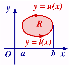
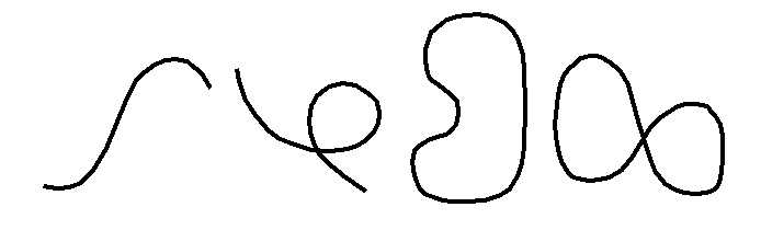
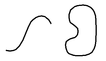
Definition A continuous arc is a set of points (x, y): x =
If functions Definition A contour is a continuous chain of a finite number of smooth arcs joined end to end.
Definition For a smooth arc, the length exists and is given by
Dividing through by
Integrating this expression with respect to t gives the required result. Note It can be shown that this formula is independent of the choice of parameter used. Let C be a contour extending from z = Let f(t) = u(t) + iv(t) be a (sectionally) continuous function on C (that is, the real functions u = u(t) and v = v(t) are sectionally continuous over a Definition We define
Here, Note that the line integral exists because the integrand on right is sectionally continuous.
Suppose f(z) = u + iv = u( Then substituting f(z) = u + iv in the defining expression
gives
or simply
Note In summary, Thus we have expressed the complex line integral in terms of two real line integrals.
1. 2. 3. 4. If C1 is a contour (with parameter t from 5. If C has length L and |f(z)| Properties (2) and (3) express the linearity of the integral.
Proof We use Property 5 of the Definite Integral: | Now, |
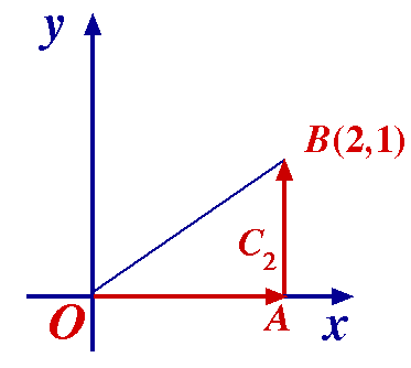
Now, z2 is continuous and on C1, z2 = (x2 – y2) + 2ixy = 3y2 + 4y2i , [strictly ( Hence I1 = Now I2 = Question 1 We see that in the previous examples, the integral from O to B is the same for both contours. Is this a coincidence? Or does it always happen? If it doesn't always happen, when does it? We can express this in a different way. We see that
So we ask: Is the integral around a closed contour always zero? Question 2 We observe that if we forget the contour altogether, and simply integrate, then we obtain:
Does this always happen? This would say that
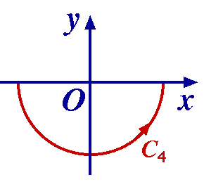
Now C3 is the contour of points (x, y) | x = cos and dz = (– sin Hence we have I3 = = =
I4 = We observe that this is different from I3! Note On the contour C, |z|2 = z
| In this case, the length L = Therefore for z on C | z4 | = (x2 + y2)2 = [ x2 + (1 – x)2 ]2 = [2x2 – 2x + 1]2. That is, | z4 | = [2(x – 1/2)2 + 1/2]2 (In retrospect, this is obvious from the figure! Why?) Hence | 1/z4 | Let R be a closed region in the real plane made up of a closed contour C and all interior points. If P(x, y), Q(x, y) are real continuous functions over R and have continuous first order partial derivatives, then Green’s Theorem says:
where C is described in the anti-clockwise direction. Outline Proof
= = –
Now consider a function f(z) = u(x, y) + iv(x, y) which is analytic at all points within and on the closed contour C, and is such that f '(z) is continuous there. We show that The given conditions tell us that u, v and their first order partial derivatives are continuous. Now
= – = 0, using Green's Theorem and the Cauchy-Riemann equations. This result was discovered by Cauchy. As a consequence of Cauchy's Theorem we have the following:
Goursat showed that Cauchy’s condition ‘f '(z) is continuous’ can be omitted. This discovery is important, because from it we can deduce that all derivatives of analytic functions are also analytic. But, proving this stronger result takes much more effort! Theorem 5.1 (Cauchy-Goursat Theorem) If a function f is analytic at all points interior to and on a closed contour C, then Now the integrand z2/(z–3) is analytic everywhere except at the point z = 3. This point lies outside the circular disk | z |
[We note that Laplace's integral can be evaluated by writing
and expressing this second integral in polar coordinates.] We integrate f(z) = exp(–z2) around the rectangle C defined by | x | Since exp(–z2) is entire, the Cauchy-Goursat Theorem applies, that is, Hence
Taking out the factor
Equating the real parts,
or
since the integrand is even. Let f be analytic in D and z0, z
Theorem 5.2 (‘Primitive’ Theorem) For all such paths in the domain D
has the same value, and F'(z) = f(z). Note This will allow us to evaluate some line integrals by straight integration. We shall see that the name of the theorem comes from the fact that the function F satisfying F'(z) = f(z) is called a primitive of f. Proof Let z + F(z + where since Now clearly on the segment,
Then Now f is continuous at z. Hence for all | Hence, when |
(using Property 5). That is,
and F(z) exists at each point of D, and F'(z) = f(z). We say that F is an indefinite integral or primitive (anti-derivative) of f and write F(z) = That is, F is an analytic function whose derivative is f(z). Since
we can use this as a means of evaluating line integrals.
|
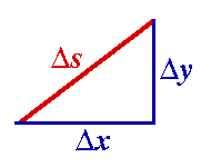 Now, where does this strange formula come from? From Pythagoras' Theorem, the length
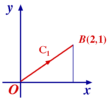
 , again!
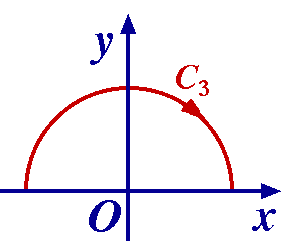
 In this case we obtain
 We make use of Property 5: